Estimating Tsunami Travel Times

Want to know how long you have until a tsunami generated in Chile reaches your doorstep? To figure it out you need two things: the speed of the wave generated and the great circle distance between you and the location of tsunami origin.

Wave speed (c) is related to the depth (H) of the water body the wave is moving through:

c = √(gH)

 

where g is acceleration due to gravity = 9.8 m/s² and H is in meters. The average wave speed in open ocean is approximately 200 m/s. This is fine to use in back of the envelope calculations such as this.

 

To find the great circle distance between two points you need the radius of the earth (approximately 6370 km) and the spherical angle (ψ) between the points, given by: 

ψ = arcos [ sin(φ₁)sin(φ₂) + cos(φ₁)cos(φ₂)cos(θ₂ – θ₁) ]

where φ₁ and φ₂  are the latitudes of the starting and ending points respectively. θ₁ and θ₂ are the longitudes of the starting and ending points respectively.

From there, use the spherical angle and radius to find arc length (s): s=rψ. Once you have that, you can find the travel time of the tsunami: t = s/c. Keep in mind that this is very general and rough!

I've generated a Matlab script calculating the travel time for a tsunami generated in Santiago, Chile to reach Honolulu, Hawaii (~11.5 hrs according to my script). If you want to pick different starting or ending points, just mess with the latitudes and longitudes.

Interested in tsunamis? Check out these sites:
Violent Hawaii: Deadly Tsunamis
NOAA Tsunami Website
 

%Long Gravity Wavesclose all

clear all

c = 200; % speed of propagation (m/s)
r = 6370; % radius of Earth (km)
r2 = r*1000; % radius of Earth (m)

lat1 = -35.846; % Latitude of santiago, Chile -33
lat2 = 21.467; % Latitude of Honolulu, Hawaii 22
lon1 = -72.719; % Longitude of Santiago, Chile -71
lon2 = -157.983; %Longitude of Honolulu, Hawaii -158

cosangle = sin(lat1)*sin(lat2) + cos(lat1)*cos(lat2)*cos(lon2 - lon1);

angle = (acos(cosangle))*(180/pi); % angle in degrees

arclength = 2*pi*r2*(angle/360) % arclength between locations (m)

time = (arclength/c)*(1/60)*(1/60) % travel time (hr)

  

Monte Carlo integration: How the number of iterations used affects precision

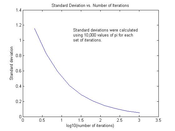
While it may be obvious that with Monte Carlo integration, the more iterations performed will result in higher precision, it's always fun to look at something graphically. Since I had already written a program that approximated the value of pi (check it out here), I decided to look at how standard deviations change with increasing numbers of iterations.

I chose to run 10 sets of iterations: 2, 4, 8, 32, 64, 128, 256, 512, and 1024. Why these values were chosen becomes obvious in the script, but you can use any set of iterations you want. Each set of iterations was run 10,000 times and standard deviations were calculated from these.

Figure 1: Stdev vs. number of iterations. Note the x-axis is log scale so that the trend can more easily be seen.

Here's my script:

% Graphing standard deviations of pi vs. number of iterations

% using Monte Carlo integration

close all

clear all

for x = 1:10;           

   

y=2^x;

   

for i = 1:10000;

    n = 2*(rand(2,y))- 1;    % generates random numbers between -1 and 1

   

    pts = 0;                  % starting value for total points

    circ = 0;                 % starting value for points within circle

   

    for R = 1:y;

        d = sqrt((n(1,R))^2 + (n(2,R))^2);

        pts = pts + 1;

        if d <= 1;

            circ = circ + 1;

        end  

    end

    Pi(1,i) = (4*circ)/pts;

end

STD(1,x) = std(Pi);

IT(1,x) = y;

end

plot (log10(IT),STD)

title('Standard Deviation vs. Number of Iterations');

xlabel('log10(number of iterations)');

ylabel('Standard deviation');

Calculating Pi: Monte Carlo Integration

Thank you physicists, Matlab, and (pseudo)random number generators. Welcome to Monte Carlo integration. A couple of days ago, my boyfriend was telling me how he has surpassed me in his Matlab skills. Dorky, I know.  Not one to be bettered, I set out to prove him wrong. He had an assignment to approximate the value of pi using Monte Carlo integration in C. I'd do it in Matlab.

But I had to figure out what Monte Carlo integration was first.

Enter Wikipedia. I don't care what professors say about it, Wikipedia is a magical place filled with more knowledge than could ever be stuffed into my head. I'm not going to start citing the website in anything important, but I will give it my thanks. So here it is: Monte Carlo integration offers an approximate evaluation of definite integrals using random numbers.   

So what did I have to do exactly? My bf gave me a hint: use a circle and a square. After some more prodding he added, "put the circle in the square." Alright. Thanks a lot.

So I drew up a circle with radius = 1, inside a square with sides = 2 (Figure 1).

Figure 1: Circle with radius = 1 within a square with sides = 2.

We know that the area of the square is L²= 2² = 4.

We know the area of the circle is
A = πr². To find π, we need to know the area of the circle. Unfortunately, that's impossible to know without π.

But there is another way to find pi. I first set the center of the circle as (0,0) in a coordinate plane. I then could generate sets of random numbers between -1 and 1 and use these as x and y coordinates. Using Pythagorean's Theorem I can find the distance of these points from the center (the origin):

c = √(a² + b²).

If a point's distance from the origin is < 1, then it falls within the circle. The ratio of points within the circle to the total number of points (points within the square) is proportionate to the ratio of the area of the circle to the area of the square:

                                               # points in circle   =    πr²           where r=1

                                                # points total             4

So:    

                                              π    =    4(# points in circle)

                                                              # points total

With that in mind, my Matlab adventure began.

The script was pretty easy to write (find it at the bottom of this page). The hardest part for me was actually plotting the figure. Obviously, the more iterations (# of points) you do, the more accurate your result will be (Table 1). It also vastly increases the computing time. Past 1,000,000 iterations, my Matlab program got pissed and said it didn't have enough memory.

# of Iterations	Approximate value of Pi
10	2.4
100	3.24
1000	3.092
10000	3.1104
100000	3.13168
1000000	3.143080

                            

Here's my Matlab script for 1000 iterations:

% Calculating pi using Monte Carlo integration

close all

clear all

n = 2*(rand(2,1000))- 1;        % generates random numbers between -1 and 1

t=sum(n.*n,1)<1;

pts = 0;                       % starting value for total points

circ = 0;                      % starting value for points within circle

for R = 1:1000;

    d = sqrt((n(1,R))^2 + (n(2,R))^2);

    pts = pts + 1;

    if d <= 1;

        circ = circ + 1;

    end

end

format long

Pi = (4*circ)/pts

plot(n(1,~t),n(2,~t),'b.','MarkerSize',15)

hold on

plot(n(1,t),n(2,t),'r.','MarkerSize',15)

theta = linspace(0,2*pi,100);    

x = cos(theta);                 

y = sin(theta);                  

plot(x,y,'k'); 

axis ('equal');

axis([-1 1 -1 1]);

title('100 Iterations');